My experiments with growing a fractal

I started learning Mojo by implementing diffusion-limited aggregation (DLA) and experimenting with ways to make it faster.

What’s DLA?

DLA grows a cluster through successive random walks. Starting from a seed, each new particle walks from the grid’s edge until it reaches an empty cell adjacent to the cluster, where it sticks.

seedParticle() // Usually a single particle at the center.
For each new particle:
    Sample an empty boundary cell uniformly.
    Random-walk until adjacent to the cluster.
    Attach the particle.

These local rules produce the branching fractals below. The pattern emerges as particles accumulate.

Stickiness sets the chance of attachment at each contact check. At 1.0, contact always leads to attachment. At 0.1, each check has a 10% chance to attach; otherwise, the particle attempts another step. Lower stickiness lets particles explore beyond their first contact.

Here, the walk uses four equally likely directions on a finite grid. A move outside the grid or into the cluster leaves the particle in place. Every speed comparison below uses stickiness 1.0, so all methods solve the same growth problem.

How do we simulate it?

1. Brute force: follow every step

My first implementation did exactly what the animation shows: spawn a particle, simulate its random walk, and stop when it sticks. Then start the next one.

It worked, and it was already quite fast. But a particle could spend thousands of steps in empty space before finding the cluster. I only needed its final sticking position. Could I get that without simulating the whole walk?

2. Compute the possible outcomes, then sample one

The next particle can only stick in an empty cell beside the cluster. My thought was to list those cells, compute the chance of ending up at each one, and sample from that distribution.

I arrived at this idea while working through the problem, then found that calculating the DLA attachment distribution by solving the Laplace equation has a long history. Hayakawa, Sato, and Matsushita (1987), for example, calculate the distribution over perimeter sites this way. My version uses the launch and boundary rules of this finite grid.

Each new particle changes the cluster and the distribution of where the next one will stick. To calculate that distribution, the matrix method combines the effect of all possible walks, including detours and returns, into a system of equations. Solving it gives a weight for each neighboring cell.

Find the empty cells where a particle could stick.
Build equations from the possible moves through the grid.
Solve for the attachment distribution over those cells.
Sample one cell from the distribution and add it to the cluster.
Calculate the new distribution before adding the next particle.

Calculating the distribution

Let $T$ contain reachable wandering cells and $A$ the sticking cells. $Q$ gives one-step probabilities from $T$ to $T$ ; $R$ gives those from $T$ to $A$ . Rows describe the starting cell, and columns the destination. Split the launch distribution into $\mu_T$ and $\mu_A$ , then solve

(I-Q^{\mathsf T})g=\mu_T, \qquad p=\mu_A+R^{\mathsf T}g.

Here $I$ is the identity matrix, $g$ counts expected visits before sticking, and $p$ is the attachment distribution. The transpose collects contributions from incoming moves. The $\mu_A$ term handles particles launched beside the cluster. My Mojo implementation solves a sparse linear system; it does not construct a matrix inverse.

This skipped the walk, but it wasn’t the speedup I expected. Every attachment changes the equations, so the next particle needs another solve over the reachable empty grid.

3. Can we solve only a rectangle near the cluster?

Most of the grid was empty and unchanged. Could I put a rectangle around the cluster, solve inside it, and reuse what I knew about the outside?

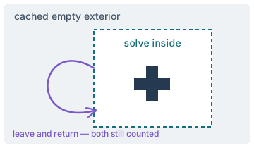
A walker can leave the inner rectangle and return through the empty exterior

The outside still matters: a walker can leave the rectangle and come back somewhere else. The rectangle method caches those effects instead of turning the rectangle into a wall. The algebra is a Schur complement, a standard reduction of a larger system. Dörfler and Bullo’s work on Kron reduction describes this operation for graph Laplacians; it supports the reduction, rather than prescribing this particular DLA implementation.

Choose a rectangle enclosing the cluster and its sticking cells.
Compute and cache how the empty exterior affects that rectangle.
Solve the smaller system inside, including those exterior effects.
Sample the next attachment; rebuild the cache when the rectangle grows.

The rectangle's exact reduction

Partition the linear system into an interior $I$ and exterior $E$ . Eliminating the exterior variables gives

(A_{II}-A_{IE}A_{EE}^{-1}A_{EI})x_I =b_I-A_{IE}A_{EE}^{-1}b_E.

Both the operator and the source change. The implementation obtains these terms through solves, not stored inverses. The cached exterior remains reusable while its geometry is unchanged.

The smaller solve came with another cost: preparing and rebuilding that cache. In my measured implementation, the rectangle method was slower than the full-grid matrix method.

4. What if the GPU does the solve?

I next tried moving the matrix solve to the GPU. The particles still attach one at a time; the parallel work is the linear algebra for each particle.

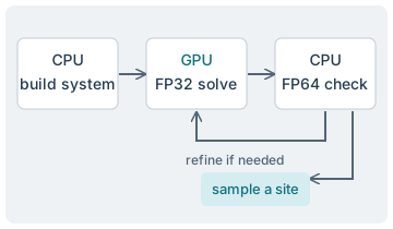
Build the system on CPU, solve in 32-bit precision on GPU, then check and refine in 64-bit precision on CPU

The GPU computes in 32-bit precision, then the CPU checks and refines the answer in 64-bit precision. My implementation also creates buffers and transfers data for each particle. On the small workload below, those costs left it slower than the CPU solver. Moving the calculation to different hardware hadn’t removed the repeated work.

5. Take a step back: skip only the empty wandering

Instead of predicting where the entire walk ends, could I predict where it leaves a small empty region?

That’s the square-exit approach. Center a square on the walker, with no sticking cells inside it. Sample where the walker first reaches the square’s boundary, jump there, and carry on.

No sticking can happen inside that square, and future moves depend only on the exit cell. So a correctly weighted jump preserves the eventual attachment distribution, up to numerical rounding. Choosing a random perimeter cell uniformly would give the wrong weights.

Choose a square around the particle with no sticking cells inside.
Keep the square inside the grid.
If there's enough room, sample an exit from a precomputed table.
Near the cluster, take ordinary steps and check whether to stick.
Continue until the particle sticks.

The walk-to-square method in Loh (2014) describes this shortcut. I use its local exit idea within my finite-grid rules. Mojo computes tables for reusable square sizes at compile time; a saved distance-to-cluster map helps choose a safe square at runtime.

This was the useful change: solve a small, reusable exit-distribution problem instead of solving the whole changing grid for every particle.

Watch the five methods at real-time speed

One second of replay equals one second of measured computation. Each method gets the same 101 × 101 grid, 200 particles, and full stickiness. Runs were recorded separately to avoid competing for the machine; the replay puts them on one clock.

Open the five-method video directly

The first eight seconds, looping at 1×. Seed 42; full grids, identical scale. Finished panels freeze until the loop restarts. The two walk methods finish in a fraction of a second—there is no slowdown to make them easier to see. On a phone, use fullscreen for the panel labels.

Method	Median time	Range over five seeds
Random walk · CPU	0.117 s	0.105–0.141 s
Matrix · CPU	14.60 s	13.92–14.88 s
Rectangle · CPU	23.80 s	23.25–24.46 s
Matrix · GPU	26.74 s	24.95–27.43 s
Square exits · CPU	0.017 s	0.015–0.017 s

The median is the middle of five timings. On this workload, the global solves and cache preparation cost more than walking. The GPU is slower than the CPU solver here; this small-grid experiment does not tell us where that tradeoff reverses.

Full measurements · Source and reproduction instructions

A seed makes the random-number sequence repeatable. Different algorithms consume that sequence differently, so their pictures need not match. Visual resemblance is not a correctness test.

Measurement details and the larger-grid result

Apple M3 Pro, 36 GB; Mojo 1.2.0, -O3; five seeds (42–46), with method order rotated. The video uses seed 42, chosen before measurement. Each run starts a fresh process and grid. Times cover the public spawn-and-stick call, including cache builds, GPU setup, transfers, and CPU refinement. Ahead-of-time compilation, initial grid allocation, capture/export, and drawing are excluded. The GPU result is for this hybrid implementation, not a universal hardware comparison. Matrix solves are checked against a 1e-10 relative residual target; that is not a bound on every attachment probability.

On the separate 501 × 501 / 2,000-particle workload, random walk’s median was 38.31 s, versus 1.10 s for square exits (about 35×). That larger-grid result measures only those two methods and should not be merged into the five-method ranking above.

Open the larger-grid video directly

An eight-second loop at 1×, ending before random walk finishes. The full seed-42 runs take 38.12 s versus 1.26 s; those individual times differ from the five-seed medians. Both panels show the same central 251 × 251 crop; every attached particle remains visible.

Large-grid measurements · Reproduce both experiments

The lesson I want to keep

The matrix method skips an entire path but pays for a global solve. Square exits reuse a small local solution many times. Choosing which outcome to compute mattered as much as choosing where to run the computation.

Random walk and square exits also support the partial stickiness introduced at the start. The current matrix variants require full stickiness.

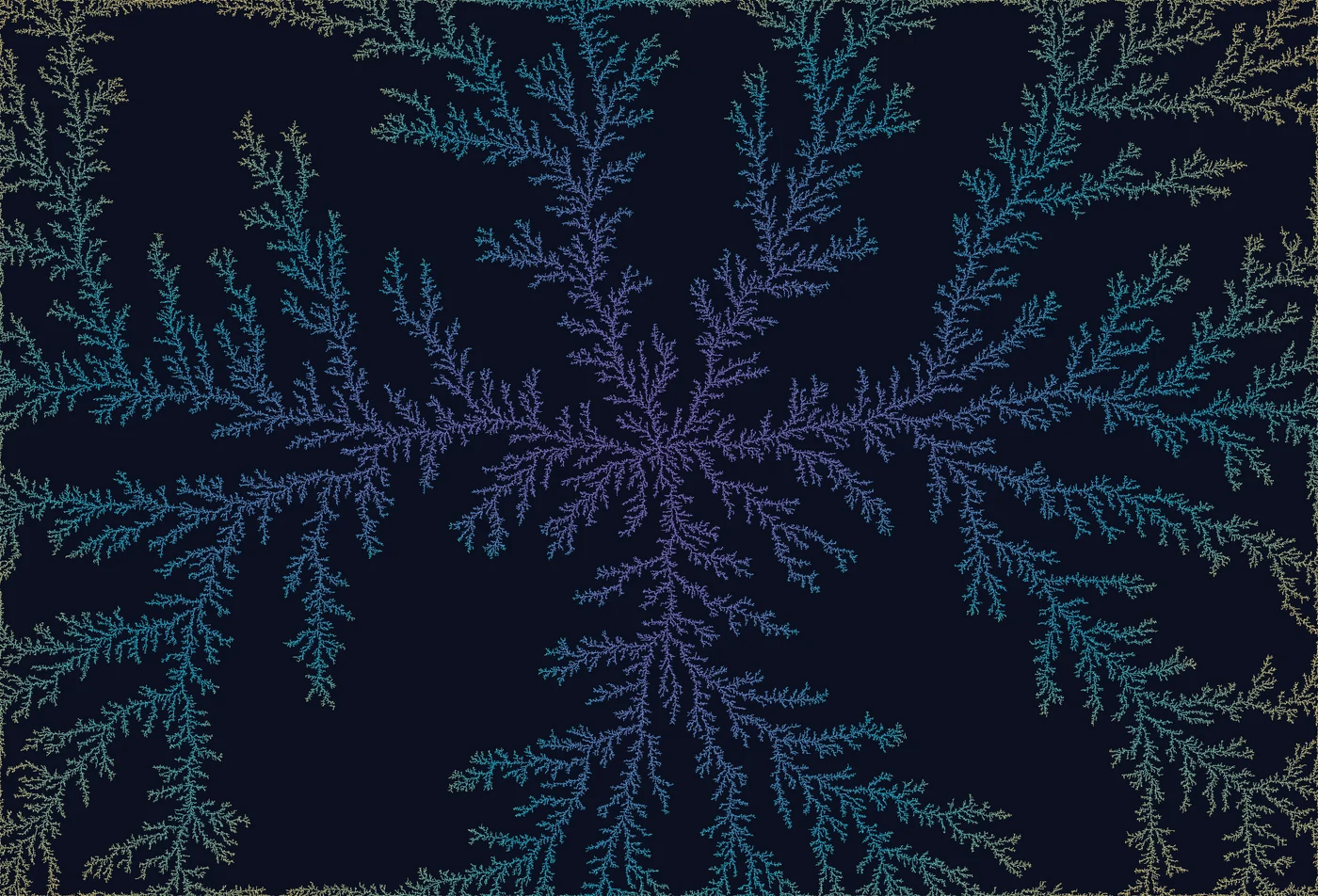
A larger DLA run, with older branches in violet and newer tips in cyan and gold.

One of the larger runs became my wallpaper. Same small growth rule; many repetitions.